Theory-Inspired Parameter Control Benchmarks for DAC

Accompanying blog post for our GECCO'22 paper

NOTE: We are using pyscript for the example below. Loading might take a bit longer.

LeadingOnes:

Steps Taken:

Speed: 1% Number of bitflips: 1

${\color{gray}(1+1)}$RLS on a randomly initialized LeadingOnes problem. You can manually configure how many bits get flipped in each iteration via the lower slider. We only render the current best solution, thus some steps might not change the image. Cells that will not change anymore are colored in green. For pseudocode see Algorithm 1.

To achieve peak-performance on a problem, it is often crucial to correctly setup, i.e. configure, the algorithm which is supposed to solve the problem. In many communities it has been observed that fixed parameter choices are often not optimal and that dynamic changes to parameter during the algorithms run can be highly beneficial (see, e.g., ). The evolutionary algorithms community is no stranger to this observation. Under the heading of parameter control (for an overview see ) various methods have been proposed to adapt parameters on the fly. More importantly however, the community has provided various theoretical insights.

In a similar vain to parameter control, the novel dynamic algorithm configuration (DAC) framework proposes to learn parameter adaptation policies in a dedicated offline learning phase. Once a policy was learned, it can then be used to adapt algorithm parameters on a variety of problem instances. Still, the field is very young and there is much to learn. In our recently accepted GECCO paper Theory-Inspired Parameter Control Benchmarks for Dynamic Algorithm Configuration builds on such insights of the parameter control community to build benchmarks which can be used to evaluate DAC methods and policies.

Why RLS on LeadingOnes?

The short answer is, LeadingOnes is very well understood. The slightly longer answer is, LeadingOnes is one of the most rigorously studied problems in the parameter control community. The parameter control community has thoroughly studied the dynamic fitness-dependent selection of mutation rates for greedy evolutionary algorithms on LeadingOnes. Thus, it is very well understood how the expected runtime of such algorithms depend on the mutation rates during the run. Overall LeadingOnes is an important benchmark for parameter control studies both for empirical and theoretical analysis . Thus, this makes LeadingOnes an ideal benchmark to also study DAC methods in depth. Further, the theoretical insights can be used to provide a ground truth on LeadingOnes. This was not possible for prior DAC benchmarks , besides some manually designed artificial benchmarks.

A Short Primer on LeadingOnes and RLS

If you are already familiar with the LeadingOnes problem you can skip this short introduction. LeadingOnes is perfectly named. For a bitstring of length $\color{gray}n$, the LeadingOnes problem is to maximize the number of uninterrupted leading ones in the bitsring.

There are a variety of algorithms one could use for solving LeadingOnes. Here, we chose to use $\color{gray}(1+1)$RLS. The pseudo code for this is:

def RLS(problem_dimension, max_budget):
    partial_sol = numpy.random.choice(2, problem_dimension)
    for t in range(max_budget):
        s = get_current_state()
        num_bits_to_flip = policy(s)
        new_partial_sol = flip(partial_sol, num_bits_to_flip)
        if fitness(new_partial_sol) >= fitness(partial_sol):
            partial_sol = new_partial_sol

Algorithm 1: Pseudocode for ${\color{gray}(1+1)}$RLS

The algorithm starts from a randomly initialized bitstring and in each iteration randomly flips num_bits_to_flip. The so created new solution candidate is compared to the old one. The old one is replaced by the new one if the latter one is not worse than the former one. When using an algorithm for solving the LeadingOnes problem, we are interested in setting the algorithm up such that we solve the problem using as few function evaluations as possible, or in other words in as few iterations as possible. At the top of this post you can find a working implementation of this setup where you are in charge of setting the number of bits to flip in each iteration. If you’ve played around with this setting a bit, you might have noticed a few things:

A too high number of bits to flip becomes detrimental the more leading ones we have.
Always only flipping one bit is a valid strategy but might take a long time (depending on the initialization).
Decreasing the number of bits to flip over time fairly reliably reduces the required running time.

Ground Truth and Optimal Policies

It was proven that we can compute the probability of improving the current partial solution of length $\color{gray}n$ with fitness value $\color{gray}i\leq n$ by flipping $\color{gray}r$ bits as $\color{gray} q(r,i)=\frac{r}{n}\cdot\prod_{j\in\left[1,\ldots,r-1\right]}\frac{n-i-j}{n-j}$. Further, an optimal policy that can choose to flip any number of bits in $\color{gray}\left[1,\ldots,n\right]$ satisfies $\color{gray}\pi_{\text{opt}}\colon i\mapsto\lfloor n/(i+1)\rfloor$. Thus, if our current solution has fitness $\color{gray}0$ (i.e., no leading ones) we should flip all bits. If we only have one leading one, we should flip exactly $\color{gray}\lfloor n/2\rfloor$ bits, and so on. Let’s compare this optimal policy to static ones:

Optimal Policy:

$\color{gray}\pi_{\text{opt}}($

$\color{gray})\mapsto$

LeadingOnes:

Steps Taken:

#Solved:

$\color{gray}\mu_{\text{steps}}$:

Static Policy:

LeadingOnes:

Steps Taken:

#Solved:

$\color{gray}\mu_{\text{steps}}$:

Speed: 1% Number of bitflips: 1

We can see that the optimal policy is quite a bit faster at solving the LeadingOnes example. However, what about policies that are restricted and cannot choose from all values in $\color{gray}\left[1,\ldots,n\right]$? In our paper, we present a method to compute the optimal policy for any such restricted choice. In essence, we can use the probability of improvement as defined above and only need to compare the probability of consecutive elementsWe assume the portfolio is always sorted. of the portfolio. Whenever we have a higher probability of improvement with the smaller portfolio element, we switch to that. So, for any $\color{gray}n$ and portfolio $\color{gray}\mathcal{K}$ we can compute the optimal policy and thus generate ground-truth about the behaviour of $\color{gray}(1+1)$RLS.Note that 1 always needs to be included as we otherwise can't guarantee that a solution will be found. This ability to compute the optimal policy for any portfolio (i.e., configuration space) makes this setting ideal to study how different problem sizes and configuration spaces influence DAC methods.

Learning DAC Policies

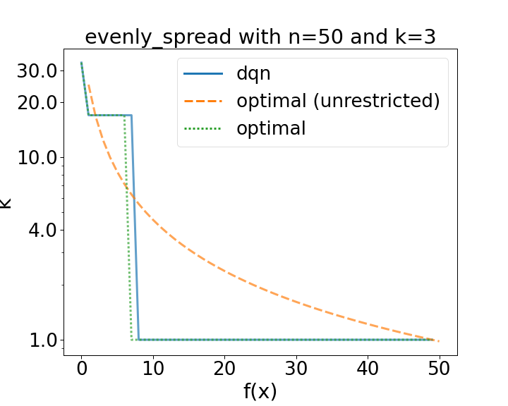
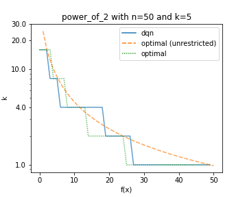
Now that we know all about the benchmark, lets use it to gain insights into a DAC methodIf you need a lightweight introduction to DAC we refer to . To give an example of the use-case of this benchmark we train a small DDQN agent to dynamically configure the number of bit flips of RLS on LeadingOnes based on the observed fitness value.

Comparison of a learned policy (dqn) compared to optimal ones. The dotted green line used the same restricted configuration space as the DQN. (left): The configuration space consists of three evenly spread values [1, 16, 32]. (right): The configuration space consists of five values [1, 2, 4, 8 16].

Our first results (shown in the figures above) show that the DQN is indeed capable of learning optimal policies. Indeed on the same restricted configuration space for bitstrings of length 50, the DQN quickly learns the to play the optimal policy or ones that result in virtually the same reward.

The availability of ground truth however not only enables us to compare the learned performance to the known optimal one, we can also study the limits of the chosen DAC method. For example, we can evaluate how the same DQNs learning capabilities scale with the size of the configuration space.

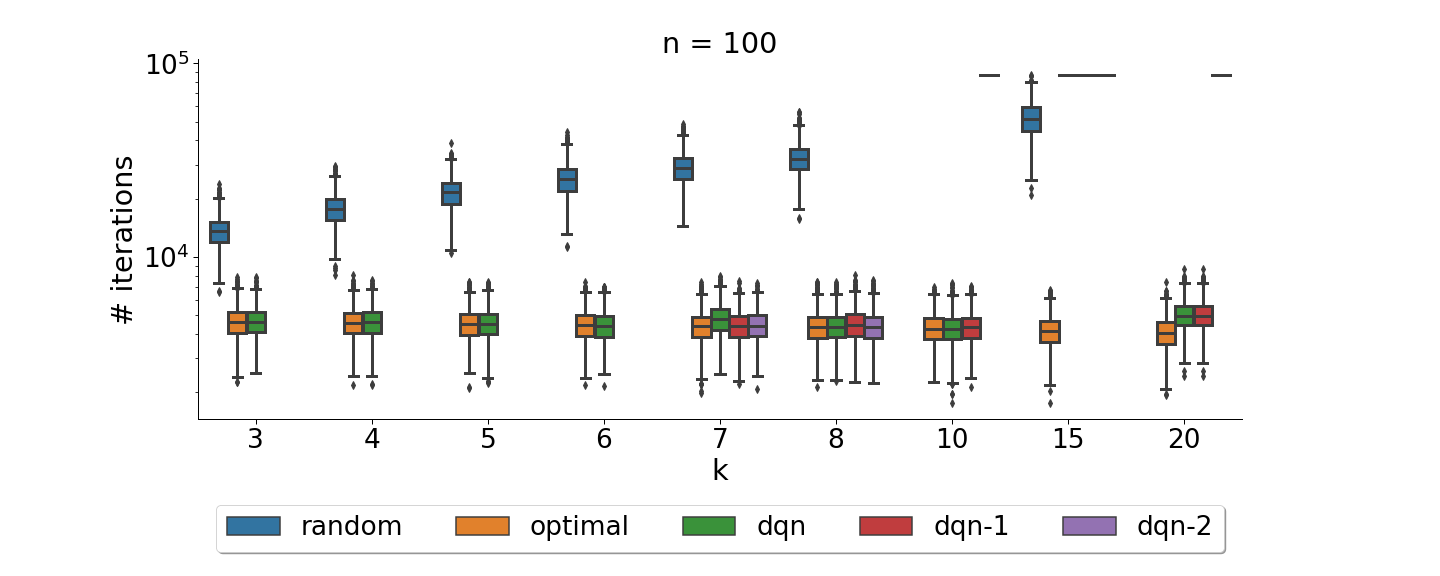
Comparison of a learned policy (dqn) compared to optimal and random ones on problems of size 100 with varying portfolio sizes. For $\color{gray}k\geq7$ we plot three distinct runs to highlight the increased instability of DQN. For $\color{gray}k = 15$ none of the dqn runs were capable of learning meaningful policies.

Overall we could observe that the chosen DAC method, with its used parameter settings was capable of learning optimal policies but struggled to scale to larger action spaces as well as portfolio sizes. For more details we refer the interested reader to our paper.

Conclusion

Our work presents a novel benchmark that is useful for both parameter control and DAC research. The benchmark fills an important gap in the existing benchmarks for DAC research as it enables us to compute optimal policies. We thus can easily evaluate the quality of learned DAC policies and as well as DAC techniques themselves. We showed how we can use the benchmark to gain insights into a DAC method and explored settings in which the chosen DQN method started to break down. We hope that our work is the first of many exchanges of benchmarks between the parameter control and dynamic algorithm configuration communities. With the growing literature on parameter control and its theoretical analysis we hope to provide other use-cases with a known ground truth.

Our code and data are publicly available at https://github.com/ndangtt/LeadingOnesDAC and the benchmark has recently been merged into DACBench. For feedback or questions, feel free to reach out to us.